Linear Regression with TensorFlow on TimeSeries Data
Published:
In my paper on Linear Regression (see Paper 2 ) we talked about developing a Linear Regression Model for timeseries data. Our group decided to use the Adam Optimizer and Gradient Descent models to compare the results from each. This code will go over the Adam Optimizer model. Lets go over the python! You can see the full python file here: linear_regression.py
Let’s include our libraries
import tensorflow as tf
import pandas as pd
import matplotlib as mpl
mpl.use('TkAgg')
import matplotlib.pyplot as plt
import time
And make some initial variable declarations, we adjusted these during development (you can too)
batch_size = 32
learning_rate = 0.003
n_epoches = 6000
We were provided this data for our project, so we had to read it in and do some formatting. We also split the data into training and test data for the model.
training_set = pd.read_excel('/Users/krystofe/Desktop/timeseries.xlsx', header=None, names=['features','labels'])
df1 =  pd.DataFrame({'features' : training_set['features'].values, 'labels' : training_set['labels'].values})


# splitting the data into train and test dataframes
train_d = df1.sample(frac=0.7, random_state=101)
test_d = df1.drop(train_d.index)

# converting train and test dataframes to matices to create datasets
train_d = train_d.astype('float32').as_matrix()
test_d = test_d.astype('float32').as_matrix()

# creating datasets
train_dset = tf.data.Dataset.from_tensor_slices((train_d[:,0], train_d[:,1]))
test_dset = tf.data.Dataset.from_tensor_slices((test_d[:,0], test_d[:,1]))

# combining consecutive elements of the train dataset into batches
train_dset = train_dset.batch(batch_size)

# creating an (uninitialized) iterator for enumerating the elements of the dataset with the given structure
iterator = tf.data.Iterator.from_structure(train_dset.output_types, train_dset.output_shapes)
train_init = iterator.make_initializer(train_dset)

# get_next() returns a nested structure of `tf.Tensor`s containing the next element
X, Y = iterator.get_next()
We wanted to see the results of our model so we included an R^2 calculation here
def R_squared(y, y_pred):
    '''
    R_squared computes the coefficient of determination.
    It is a measure of how well the observed outcomes are replicated by the model.
    '''
    residual = tf.reduce_sum(tf.square(tf.subtract(y, y_pred)))
    total = tf.reduce_sum(tf.square(tf.subtract(y, tf.reduce_mean(y))))
    r2 = tf.subtract(1.0, tf.div(residual, total))
    return r2
Okay lets setup the Model and our linear regression variables
# Model
w = tf.Variable(tf.truncated_normal((1,), mean=0, stddev=0.1, seed=123), name='Weight')
b = tf.Variable(tf.constant(0.1), name='Bias')
y_pred = tf.multiply(w, X) + b

# Cost function
loss = tf.reduce_mean(tf.square(Y - y_pred), name='Loss')

# training
optimizer = tf.train.AdamOptimizer(learning_rate).minimize(loss)
Just because I was curious how long it took to train on the given dataset I setup the python timer around our training.
start = time.time()

sess = tf.Session()
sess.run(tf.global_variables_initializer())

for epoch in range(n_epoches):
    sess.run(train_init)
    try:
        # Loop until all elements have been consumed
        while True:
            sess.run(optimizer)
    except tf.errors.OutOfRangeError:
        pass

end = time.time()
Lets take a look at the results. On average I was getting and R^2 value for the training data of 0.032 or 96% which is pretty good for our analyses of this data.
w_curr, b_curr = sess.run([w,b])
y_pred_train = w_curr * train_d[:,0] + b_curr
y_pred_test = w_curr * test_d[:,0] + b_curr

r2_train = R_squared(train_d[:,1], y_pred_train)
r2_test = R_squared(test_d[:,1], y_pred_test)

print('R^2_train:', sess.run(r2_train))
print('R^2_test:', sess.run(r2_test))
print('elapsed time:', end - start)
sess.close()
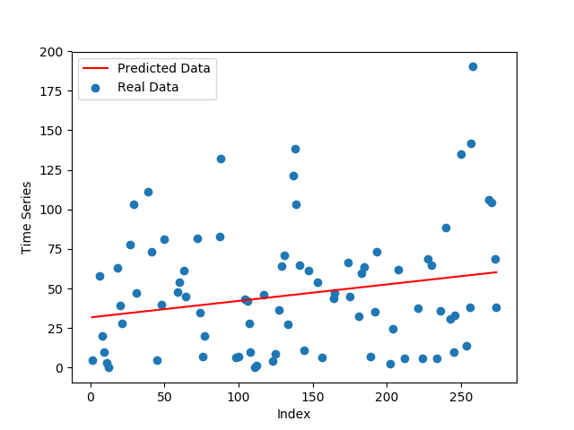
And finally lets take a look at our plots with the predictions
plt.scatter(test_d[:,0], test_d[:,1], label='Real Data')
plt.plot(test_d[:,0], y_pred_test, 'r', label='Predicted Data')
plt.xlabel('Index')
plt.ylabel('Time Series')
plt.legend()
plt.show()

